Introduction to Model-Based Thinking
Understanding Model-Based Qualitative Systems Modeling
Most engineers working in the space arena are typically trained in electrical, mechanical, or aerospace engineering. Hence, most of them understand detailed quantitative drawings and quantitative models, such as solving a circuit with Kirchhoff’s Laws to find a particular voltage in a circuit or drawing a free body diagram to solve for forces in a static mechanical system. This kind of modeling is valuable for understanding the behavior of a circuit or system in both a physical and mathematical manner. Quantitative simulation tools such as LTSpice or MATLAB can also to help evaluate these kinds of models when they get too complicated to solve by hand.
However, when the scale of a system becomes so complex that quantitative tools are cumbersome to use, the tools are less useful for design and/or analysis. Examples include an integrated circuit with so many transistors that it would take weeks for an LTSpice simulation to run. Quantitative tools are also less useful when there are many kinds of physical domains (e.g., mechanical, electronic, optical in the same system) such as for spacecraft or self-driving cars. These tools are also less useful if there a lot of software is managing the system’s behavior (for example, millions of lines of code in an airplane). A second practical issue is that during the beginning of the design cycle, many of the physical parameters needed for quantitative modeling are unknown because the design is in flux. In these situations, qualitative system modeling is more useful.
System models tend to be qualitative and logical, rather than physical and numerical, because the computational cost of modeling components numerically increases steeply with the number of components being modeled in the same simulation. In this chapter we use an op amp integrator to demonstrate the differences between quantitative and qualitative models. It is not necessary to follow the math, but it can help provide a more wholistic understanding of the processes. A qualitative representation of a system is the approach taken in the System Engineering Assurance Modeling platform (SEAM), which is discussed in this manual. This chapter is meant to help people trained in quantitative modeling make a transition to qualitative system modeling. We will first build a quantitative model of the integrator circuit, then build a qualitative model of the same circuit using standard system modeling diagrams. The purpose of this chapter is to help transition people with backgrounds in specialized engineering of science to SEAM.
Before getting into the example, we should investigate reasons for using a model-based approach to system models. We have already mentioned two reasons, namely, that modern systems, such as satellites or robots are too complex to simulate the whole system numerically, and that many of the physical parameters needed for quantitative models are unknown early in the design cycle. We can add a third reason, which is that modern engineering is making a transition from “document-based system engineering” (DBSE) to “model-based system engineering” (MBSE). In other words, instead of specifying a system and capturing all the information about the system in documents, design engineers are moving toward capturing all the specifications and information about the system in digital (software) objects, which are stored in a central repository. This helps solve one of the toughest problems of large organizations designing complex systems, which is to make sure every person working on the system is operating from the same specifications and level of information about the system at a given time (often called “versioning”). Prior to MBSE, keeping track of design changes and document versions was a huge problem for large research and development organizations. People in different departments, or different physical locations, could be working from different document versions. This would result in mistakes and unnecessary work to correct them. This approach is called “Multiple Sources of Truth (MSOT). Under the MBSE paradigm, new versions are instantly created when a change is made and are available to everyone, and old versions can be stored for reference. This idea of a “single source of truth” (SSOT) available to everyone working on the system is one of the great benefits of an MBSE approach to documenting system designs.
An Example of Quantitative Physical-Law Based Systems Modeling
A small-scale example to illustrate these points about quantitative and qualitative modeling can be seen in Figure I.1 , which shows an ideal inverting amplifier circuit configured so that the output is the integral of the input. We can use equations based on physical laws to relate the variables we see in the circuit. For example, we know that the voltage is related to the current through the capacitor by an integral expression:
Likewise, we can invoke the ideal property of the op amp that the feedback in the op amp circuit always adjusts the voltages at the op amp input terminals to be zero, so . That allows us to write the current in terms of the input voltage .
We can insert this expression into our original expression and use the fact that to write the final expression for the output voltage.
Hence if we can set the initial condition on the capacitor voltage to zero (just put a switch across it), we can obtain an ideal integral relation between the output and the input voltages.
This example is the kind of modeling familiar to most engineers. It begins with a detailed physical description of the system (the circuit schematic, in this case). The interaction of the components is modeled in terms of equations derived from physical laws. Since the model is equation-based, we could also simulate the circuit using a numerical simulator that solves differential equations. This circuit would probably be included in a larger circuit, maybe included in an integrated circuit, which itself would be on a circuit board, which might be part of an assembly of several circuit boards and electromechanical parts, such as motors. Hence this approach is a bottom-up system description.
However, when we consider large engineered systems such as automobiles or spacecraft, at some point the complexity of the system exceeds what can be modeled in this quantitative way. For one thing, even with modern computing power, the system gets too complex to be analyzed or simulated in this quantitative way. In addition, we may not know with precision all the values of all the possible physical variables that are necessary for a detailed quantitative description of a large engineered system. Lastly, such a complex physical representation is too complicated for one human being to understand and make decisions about the inter-relationships of the subsystems.
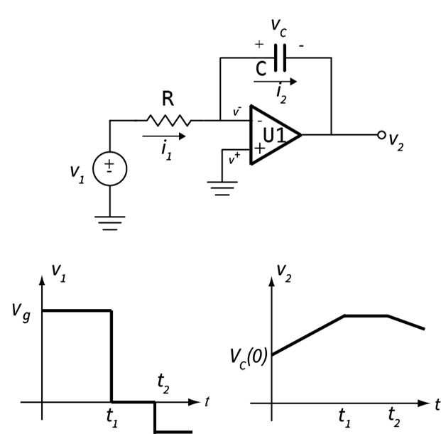
Figure I.1. An ideal op amp integrator circuit, with the input and output voltage waveforms.
The First Model-Based System Representation: The Block Diagram
In contrast to physical modeling, model-based thinking is less about mathematical relationships between components and more about the arrangements of components in the system and the functions of components and subsystems, i.e., what they are actually supposed to do. These are sometimes called “logical models,” not because they are based on digital logic, but because they are based on the logical relationships between components and the flow of signals and power through the system. Hence these modeling languages describe the system in terms of various diagrams intended to describe the form, function, and relationships of various parts of the system.
The systems-modeling part of SEAM is based on a language called SysML, which is short for Systems Modeling Language1. SysML consists of a set of descriptive diagrams that capture various aspects of the system. Let’s look at one of the most basic diagrams of SysML, the block diagram. In the block diagram we are not trying to describe detailed connections and behavior of a sub-system the way the schematic of the integrator circuit does. Rather, we just want to capture the parts of the subsystem and connections between them. Unlike a quantitative circuit schematic, which has only one correct representation, a qualitative model can have multiple forms for the same sub-system, depending on what features the modeler wants to emphasize, and what level of abstraction is needed to represent the aspects of the system the modeler is interested in.
Let's look at a couple of examples of block diagrams for the integrator. The first is shown in Figure I.2. This block diagram roughly follows the configuration of the circuit schematic. However, this diagram represents the circuit at a higher level of abstraction, which means that it is simpler than the schematic and some of the detailed information is lost. We have lost the definitions of the currents and voltages, as well as the detailed connections between connections. The diagram is no longer “solvable” using equations. All that remains is some information about which components are in the system and some basic idea of how signals flow between them.
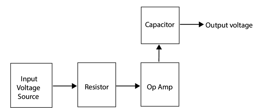
Figure I.2. Block diagram for the op amp integrator.
Now suppose that as a modeler I am interested in the signal processing aspects of the circuit. I could represent the action of the circuit by the block diagram shown in Figure I.3. There is something that creates an input signal, which is not specified, it could be a voltage source, a sensor, or another circuit. There is a block that represents the integrating action of the capacitor, which is not specified. Lastly there is a block I have labeled as "scale factor" which represents the fact that the integral is multiplied by , which produces the output signal, which could be voltage, or current, it is not specified in the diagram. Both the block diagrams in Figure I.2 and Figure I.3 are valid block diagrams of the integrator circuit schematic shown in Figure I.1, they are both higher-level abstractions of the integrator that have less information but highlight particular aspects of the integrator. In Figure I.2 the signal flow between actual components is emphasized, in Figure I.3 the signal processing aspects of the circuit are emphasized.
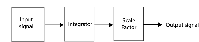
Figure I.3. Signal-processing block diagram for the op amp integrator.
The Second Model-Based System Representation: The Functional Decomposition Diagram
Now let’s look at another way to represent the system behavior, namely, a diagram that describes the relationships between a function of a sub-system and its constituent components. That is, in this diagram, we assign some “responsibility” for part of the functionality of the subsystem to each of the parts. This diagram is a key part of being able to discern the impact of a low-level failure on a top-level function.
The top-level function in our example is “Integrate the input voltage.” In Figure I.4 we have redrawn our integrator circuit to show actual components that are associated with the power source, , which is now shown to be a battery labeled , and the input signal, , which is now shown to be a light sensor based on the phototransistor, . We also assigned number values to our previous components R and C to show that in our circuit board they are specific instances of particular resistor and capacitors. In other words, R is the general symbol for a resistor, but represents a particular physical resistor of a certain value and part number from a particular manufacturer; it is the real resistor in the physical world. For example, maybe is 2 kΩ, but in the next stage of the circuit there is another 2 kΩ resistor associated with an analog-to-digital converter. Both resistors fit into the general class of 2 kΩ resistors, but physically they are different resistors, so we give them different names; let’s call the second resistor . So, the physical resistor is associated with the function of “Integrate the signal from the sensor,” but is associated with the function “Convert the analog amplifier voltage V2 to a digital code.” Now we are in a position to draw a functional decomposition diagram (), which assigns responsibility for functions to particular instances of components.
Now that we see the whole picture, we know that what the circuit is really doing is averaging the light flux illuminating the phototransistor, so we can call the system function: “Integrate the Light Flux,” or “Average the Light Flux.” Figure I.5 shows an FDD for the integrator circuit of [Figure I.4](#Figure I.4) for this system function. The top-level system function is illustrated with an upper-case F(x) symbol. The system function is divided into sub-functions (labeled with a lower-case f(x)) which are all necessary for the system function to be operational and within specification. The three sub-functions in this case are: (1) provide power, (2) sense the light, and (3) integrate (or average) the sensor signal. Each sub-function is then associated with the components “responsible” for performing the sub-function. All components associated with a sub-function must work correctly for the sub-function to be correct, unless there is redundancy built into the system (for example, two capacitors in parallel in the integrator). Now if there is a degradation or a failure in a component, we can see from the how that failure is going to propagate up to the top-level and impact the system function. For example, let’s say that the “gain,” that is, the proportionality constant between the light input and the current in the collector of the transistor, is changed because of ionizing radiation. We can see this degradation will affect both the sub-function “sense the light” and the system function “Integrate the light flux,” because the averaged light output will differ from the actual physical value because the calibration is off.
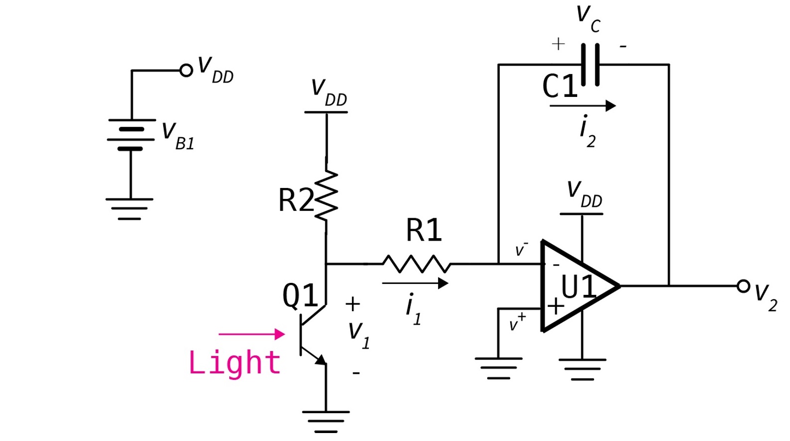
Figure I.4. Integrator showing the components associated with power and signals..
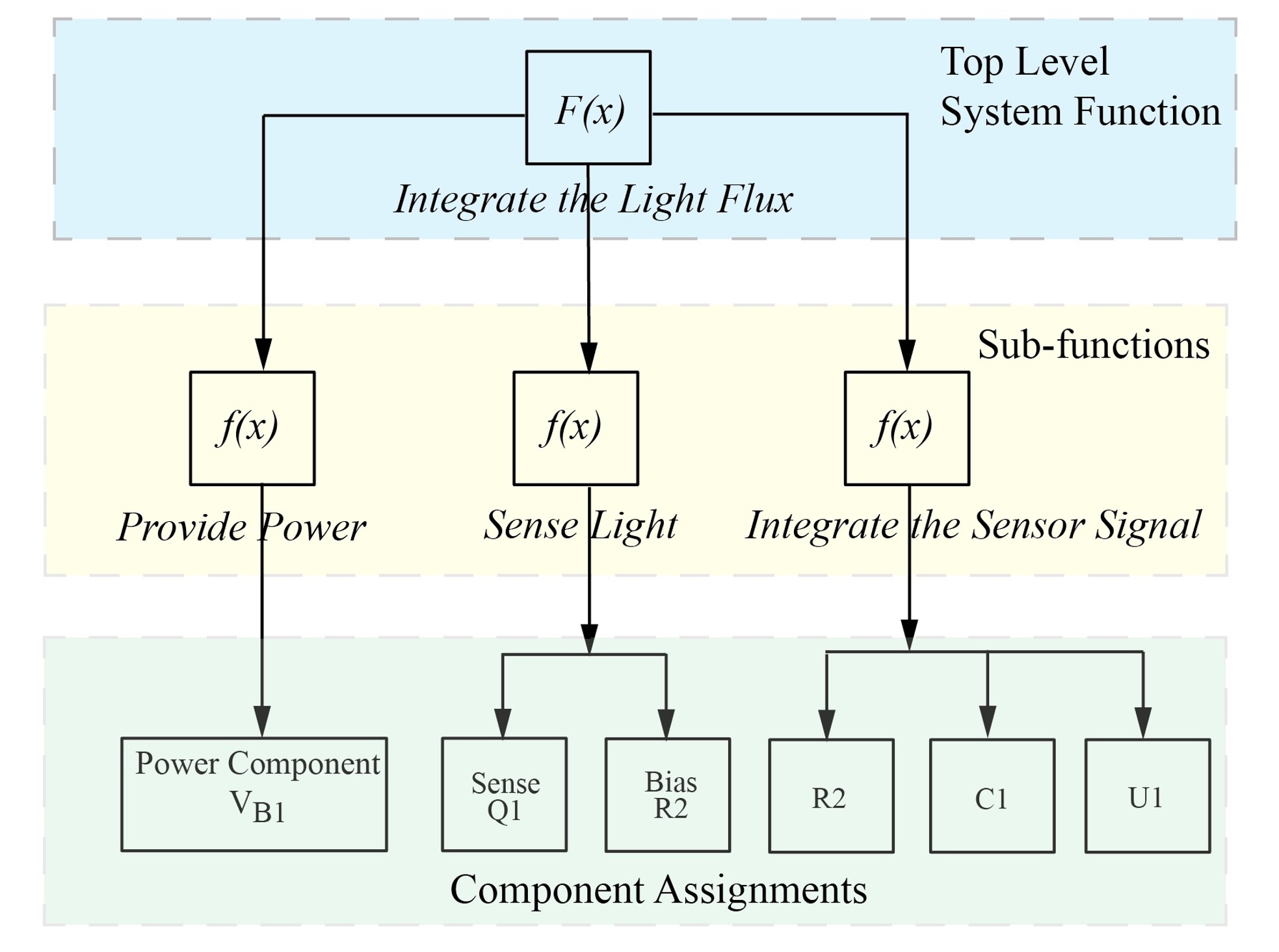
Figure I.5. Functional Decomposition Diagram for the function "Integrate the Light Flux."
- Sanford Friedenthal, Alan Moore, Rick Steiner, "OMG SysML™ Tutorial," www.omgsysml.org/INCOSE-OMGSysML-Tutorial-Final-090901.pdf, INCOSE, 2009.↩